Dear friends,

Years ago, I had to choose between a neural network and a decision tree learning algorithm. It was necessary to pick an efficient one, because we planned to apply the algorithm to a very large set of users on a limited compute budget. I went with a neural network. I hadn’t used boosted decision trees in a while, and I thought they required more computation than they actually do — so I made a bad call. Fortunately, my team quickly revised my decision, and the project was successful.

This experience was a lesson in the importance of learning, and continually refreshing, foundational knowledge. If I had refreshed my familiarity with boosted trees, I would have made a better decision.

Machine learning, like many technical fields, evolves as the community of researchers builds on top of one another's work. Some contributions have staying power and become the basis of further developments. Consequently, everything from a housing-price predictor to a text-to-image generator is built on core ideas that include algorithms (linear and logistic regression, decision trees, and so on) and concepts (regularization, optimizing a loss function, bias/variance, and the like).

A solid, up-to-date foundation is one key to being a productive machine learning engineer. Many teams draw on these ideas in their day-to-day work, and blog posts and research papers often assume that you’re familiar with them. This shared base of knowledge is essential to the rapid progress we've seen in machine learning in recent years.

That's why I’m updating my original machine learning class as the new Machine Learning Specialization, which will be available in a few weeks.

My team spent many hours debating the most important concepts to teach. We developed extensive syllabi for various topics and prototyped course units in them. Sometimes this process helped us realize that a different topic was more important, so we cut material we had developed to focus on something else. The result, I hope, is an accessible set of courses that will help anyone master the most important algorithms and concepts in machine learning today — including deep learning but also a lot of other things — and to build effective learning systems.

In that spirit, this week’s issue of The Batch explores some of our field’s most important algorithms, explaining how they work and describing some of their surprising origins. If you’re just starting out, I hope it will demystify some of the approaches at the heart of machine learning. For those who are more advanced, you’ll find lesser-known perspectives on familiar territory. Either way, I hope this special issue will help you build your intuition and give you fun facts about machine learning’s foundations that you can share with friends.

Keep learning!

Andrew

Essential Algorithms

Machine learning offers a deep toolbox for solving all kinds of problems, but which tool is best for which task? When is the open-ended wrench better than the adjustable kind? Who invented these things anyway? In this special issue of The Batch, we survey six of the most useful algorithms in the kit: where they came from, what they do, and how they’re evolving as AI advances into every facet of society. If you want to learn more, the Machine Learning Specialization provides a simple, practical introduction to these algorithms and more. Join the waitlist to be notified when it’s available.

Linear Regression: Straight & Narrow

Linear regression may be the key statistical method in machine learning, but it didn’t get to be that way without a fight. Two eminent mathematicians claimed credit for it, and 200 years later the matter remains unresolved. The longstanding dispute attests not only to the algorithm’s extraordinary utility but also to its essential simplicity.

Whose algorithm is it anyway? In 1805, French mathematician Adrien-Marie Legendre published the method of fitting a line to a set of points while trying to predict the location of a comet (celestial navigation being the science most valuable in global commerce at the time, much like AI is today — the new electricity, if you will, two decades before the electric motor). Four years later, the 24-year-old German wunderkind Carl Friedrich Gauss insisted that he had been using it since 1795 but had deemed it too trivial to write about. Gauss’ claim prompted Legendre to publish an addendum anonymously observing that “a very celebrated geometer has not hesitated to appropriate this method.”

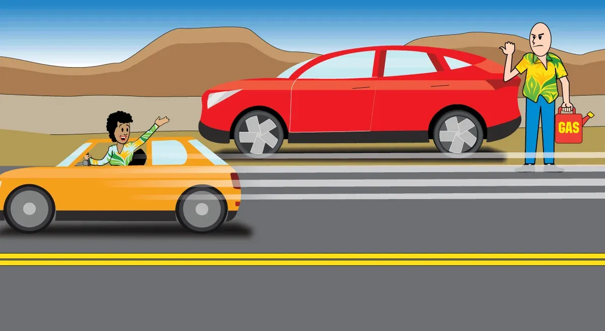
Slopes and biases: Linear regression is useful any time the relationship between an outcome and a variable that influences it follows a straight line. For instance, a car’s fuel consumption bears a linear relationship to its weight.

The relationship between a car’s fuel consumption y and its weight x depends on the line’s slope w (how steeply fuel consumption rises with weight) and bias term b (fuel consumption at zero weight): y=w*x+b.
During training, given a car’s weight, the algorithm predicts the expected fuel consumption. It compares expected and actual fuel consumption. Then it minimizes the squared difference, typically via the technique of ordinary least squares, which hones the values of w and b.
Taking the car’s drag into account makes it possible to generate more precise predictions. The additional variable extends the line into a plane. In this way, linear regression can accommodate any number of variables/dimensions.

Two steps to ubiquity: The algorithm immediately helped navigators to follow the stars, and later biologists (notably Charles Darwin’s cousin Francis Galton) to identify heritable traits in plants and animals. Two further developments unlocked its broad potential. In 1922, English statisticians Ronald Fisher and Karl Pearson showed how linear regression fit into the general statistical framework of correlation and distribution, making it useful throughout all sciences. And, nearly a century later, the advent of computers provided the data and processing power to take far greater advantage of it.

Coping with ambiguity: Of course, data is never perfectly measured, and some variables are more important than others. These facts of life have spurred more sophisticated variants. For instance, linear regression with regularization (also called ridge regression) encourages a linear regression model to not depend too much on any one variable, or rather to rely evenly on the most important variables. If you’re going for simplicity, a different form of regularization (L1 instead of L2) results in lasso, which encourages as many coefficients as possible to be zero. In other words, it learns to select variables with high prediction power and ignores the rest. Elastic net combines both types of regularization. It’s useful when data is sparse or features appear to be correlated.

In every neuron: Still, the simple version is enormously useful. The most common sort of neuron in a neural network is a linear regression model followed by a nonlinear activation function, making linear regression a fundamental building block of deep learning.

Logistic Regression: Follow the Curve

There was a moment when logistic regression was used to classify just one thing: If you drink a vial of poison, are you likely to be labeled “living” or “deceased”? Times have changed, and today not only does calling emergency services provide a better answer to that question, but logistic regression is at the very heart of deep learning.

Poison control: The logistic function dates to the 1830s, when the Belgian statistician P.F. Verhulst invented it to describe population dynamics: Over time, an initial explosion of exponential growth flattens as it consumes available resources, resulting in the characteristic logistic curve. More than a century passed before American statistician E. B. Wilson and his student Jane Worcester devised logistic regression to figure out how much of a given hazardous substance would be fatal. How they gathered their training data is a subject for another essay.

Fitting the function: Logistic regression fits the logistic function to a dataset in order to predict the probability, given an event (say, ingesting strychnine), that a particular outcome will occur (say, an untimely demise).

Training adjusts the curve’s center location horizontally and its middle vertically to minimize error between the function’s output and the data.
Adjusting the center to the right or the left means that it would take more or less poison to kill the average person. A steep slope signifies certainty: Before the halfway point, most people survive; beyond the halfway point, sayonara. A gentle slope is more forgiving: lower than midway up the curve, more than half survive; farther up, less than half.
Set a threshold of, say, 0.5 between one outcome and another, and the curve becomes a classifier. Just enter the dose into the model, and you’ll know whether you should be planning a party or a funeral.

More outcomes: Verhulst’s work found the probabilities of binary outcomes, ignoring further possibilities like which side of the afterlife a poison victim might land in. His successors extended the algorithm:

Working independently in the late 1960s, British statistician David Cox and Dutch statistician Henri Theil adapted logistic regression for situations that have more than two possible outcomes.
Further work yielded ordered logistic regression, in which the outcomes are ordered values.
To deal with sparse or high-dimensional data, logistic regression can take advantage of the same regularization techniques as linear regression.

Versatile curve: The logistic function describes a wide range of phenomena with fair accuracy, so logistic regression provides serviceable baseline predictions in many situations. In medicine, it estimates mortality and risk of disease. In political science, it predicts winners and losers of elections. In economics, it forecasts business prospects. More important, it drives a portion of the neurons, in which the nonlinearity is a sigmoid, in a wide variety of neural networks.

Gradient Descent: It’s All Downhill

Imagine hiking in the mountains past dusk and finding that you can’t see much beyond your feet. And your phone’s battery died so you can’t use a GPS app to find your way home. You might find the quickest path down via gradient descent. Just be careful not to walk off a cliff.

Suns and rugs: Gradient descent is good for more than descending through precipitous terrain. In 1847, French mathematician Augustin-Louis Cauchy invented the algorithm to approximate the orbits of stars. Sixty years later, his compatriot Jacques Hadamard independently developed it to describe deformations of thin, flexible objects like throw rugs that might make a downward hike easier on the knees. In machine learning, though, its most common use is to find the lowest point in the landscape of a learning algorithm’s loss function.

Downward climb: A trained neural network provides a function that, given an input, computes a desired output. One way to train the network is to minimize the loss, or error in its output, by iteratively computing the difference between the actual output and the desired output and then changing the network’s parameter values to narrow that difference. Gradient descent narrows the difference, minimizing the function that computes the loss. The network’s parameter values are tantamount to a position on the landscape, and the loss is the current altitude. As you descend, you improve the network’s ability to compute outputs close to the desired one. Visibility is limited because, in a typical supervised learning situation, the algorithm relies solely on the network’s parameter values and the gradient, or slope of the loss function — that is, your position on the hill and the slope immediately beneath your feet.

The basic method is to move in the direction where the terrain descends most steeply. The trick is to calibrate your stride. Too small, and it takes ages to make any progress. Too large, and you leap into the unknown, possibly heading uphill instead of downward.
Given the current position, the algorithm estimates the direction of steepest descent by computing the gradient of the loss function. The gradient points uphill, so the algorithm steps in the opposite direction by subtracting a fraction of the gradient. The fraction α, which is called the learning rate, determines the size of the step before measuring the gradient again.
Apply this iteratively, and hopefully you’ll arrive at a valley. Congratulations!

Stuck in the valley: Too bad your phone is out of juice, because the algorithm may not have propelled you to the bottom of a convex mountain. You may be stuck in a nonconvex landscape of multiple valleys (local minima), peaks (local maxima), saddles (saddle points), and plateaus. In fact, tasks like image recognition, text generation, and speech recognition are nonconvex, and many variations on gradient descent have emerged to handle such situations. For example, the algorithm may have momentum that helps it zoom over small rises and dips, giving it a better chance at arriving at the bottom. Researchers have devised so many variants that it may seem as though there are as many optimizers as there are local minima. Luckily, local and global minima tend to be roughly equivalent.

Optimal optimizer: Gradient descent is the clear choice for finding the minimum of any function. In cases where an exact solution can be computed directly — say, a linear regression task with lots of variables — it can approximate one, often faster and more cheaply. But it really comes into its own in complex, nonlinear tasks. Armed with gradient descent and an adventurous spirit, you might just make it out of the mountains in time for dinner.

A MESSAGE FROM DEEPLEARNING.AI

No advanced math required! The new Machine Learning Specialization balances intuition, practice, and theory to create a powerful learning experience for beginners. Enroll now and achieve your career goals.

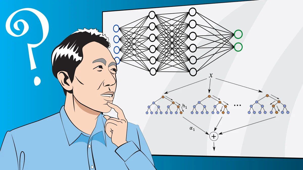
Neural Networks: Find the Function

Let’s get this out of the way: A brain is not a cluster of graphics processing units, and if it were, it would run software far more complex than the typical artificial neural network. Yet neural networks were inspired by the brain’s architecture: layers of interconnected neurons, each of which computes its own output depending on the states of its neighbors. The resulting cascade of activity forms an idea — or recognizes a picture of a cat.

From biological to artificial: The insight that the brain learns through interactions among neurons dates back to 1873, but it wasn’t until 1943 that American neuroscientists Warren McCulloch and Walter Pitts modeled biological neural networks using simple mathematical rules. In 1958, American psychologist Frank Rosenblatt developed the perceptron, a single-layer vision network implemented on punch cards with the intention of building a hardware version for the United States Navy.

Bigger is better: Rosenblatt’s invention recognized only classes that could be separated by a line. Ukrainian mathematicians Alexey Ivakhnenko and Valentin Lapa overcame this limitation by stacking networks of neurons in any number of layers. In 1985, working independently, French computer scientist Yann LeCun, David Parker, and American psychologist David Rumelhart and his colleagues described using backpropagation to train such networks efficiently. In the first decade of the new millennium, researchers including Kumar Chellapilla, Dave Steinkraus, and Rajat Raina (with Andrew Ng) accelerated neural networks using graphical processing units, which has enabled ever-larger neural networks to learn from the immense amounts of data generated by the internet.

Fit for every task: The idea behind a neural network is simple: For any task, there’s a function that can perform it. A neural network constitutes a trainable function by combining many simple functions, each executed by a single neuron. A neuron’s function is determined by adjustable parameters called weights. Given random values for those weights and examples of inputs and their desired outputs, it’s possible to alter the weights iteratively until the trainable function performs the task at hand.

A neuron accepts various inputs (for example, numbers representing a pixel or word, or the outputs of the previous layer), multiplies them by its weights, adds the products, and feeds the sum through a nonlinear function, or activation function, chosen by the developer. Consider it linear regression plus an activation function.
Training modifies the weights. For every example input, the network computes an output and compares it to the expected output. Backpropagation uses gradient descent to change the weights to reduce the difference between actual and expected outputs. Repeat this process enough times with enough (good) examples, and the network should learn to perform the task.

Black box: While a trained network may perform its task, good luck determining how. You can read the final function, but often it’s so complex — with thousands of variables and nested activation functions — that it’s exceedingly difficult to explain how the network succeeded at its task. Moreover, a trained network is only as good as the data it learned from. For instance, if the dataset was skewed, the network’s output will be skewed. If it included only high-resolution pictures of cats, there’s no telling how it would respond to lower-resolution images.

Toward common sense: Reporting on Rosenblatt’s Perceptron in 1958, The New York Times blazed the trail for AI hype by calling it “the embryo of an electronic computer that the United States Navy expects will be able to walk, talk, see, write, reproduce itself and be conscious of its existence.” While it didn’t live up to that billing, it begot a host of impressive models: convolutional neural networks for images; recurrent neural networks for text; and transformers for images, text, speech, video, protein structures, and more. They’ve done amazing things, exceeding human-level performance in playing Go and approaching it in practical tasks like diagnosing x-ray images. Yet they still have a hard time with common sense and logical reasoning. Ask GPT-3, “When counting, what number comes before a million?” and it may respond, “Nine hundred thousand and ninety-nine comes before a million.” To which we reply: Keep learning!

Decision Trees: From Root to Leaves

What kind of beast was Aristotle? The philosopher's follower Porphyry, who lived in Syria during the third century, came up with a logical way to answer the question. He organized Aristotle’s proposed “categories of being” from general to specific and assigned Aristotle himself to each category in turn: Aristotle’s substance occupied space rather than being conceptual or spiritual; his body was animate not inanimate; his mind was rational not irrational. Thus his classification was human. Medieval teachers of logic drew the sequence as a vertical flowchart: An early decision tree.

The digital difference: Fast forward to 1963, when University of Michigan sociologist John Sonquist and economist James Morgan, dividing survey respondents into groups, first implemented decision trees in a computer. Such work became commonplace with the advent of software that automates training the algorithm, now implemented in a variety of machine learning libraries including scikit-learn. The code took a quartet of statisticians at Stanford and UC Berkeley 10 years to develop. Today, coding a decision tree from scratch is a homework assignment in Machine Learning 101.

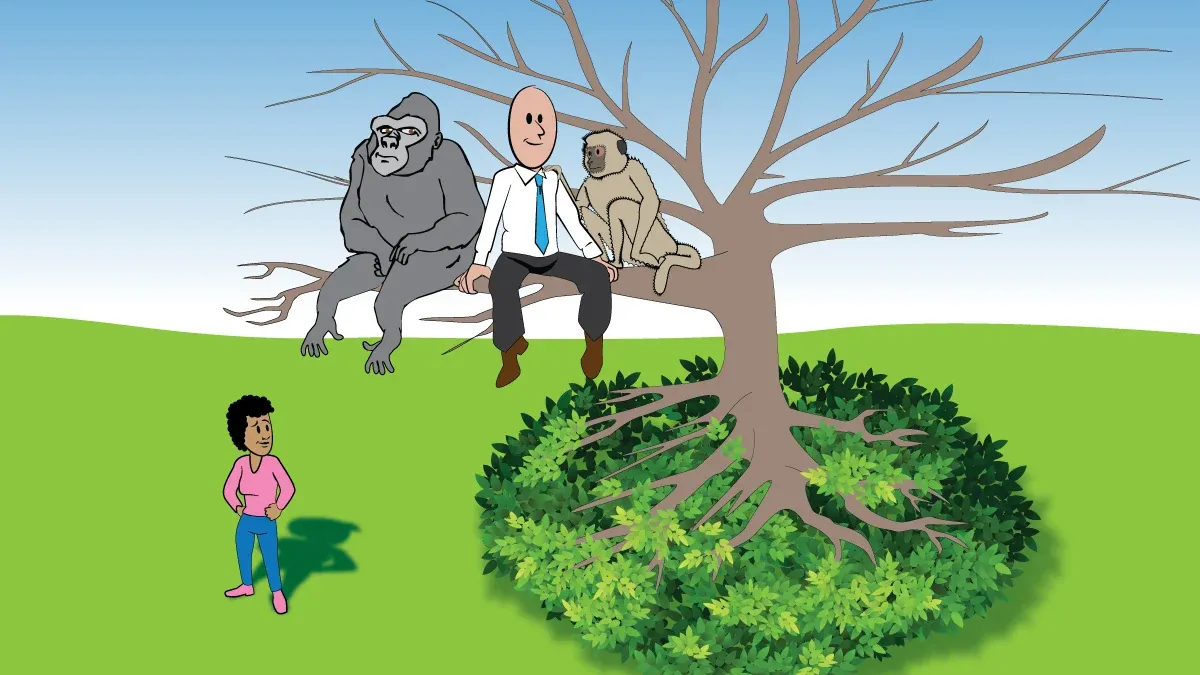
Roots in the sky: A decision tree can perform classification or regression. It grows downward, from root to canopy, in a hierarchy of decisions that sort input examples into two (or more) groups. Consider the task of Johann Blumenbach, the German physician and anthropologist who first distinguished monkeys from apes (setting aside humans) circa 1776, before which they had been categorized together. The classification depends on various criteria such as presence or absence of a tail, narrow or broad chest, upright versus crouched posture, and lesser or greater intelligence. A decision tree trained to label such animals would consider each criterion one by one, ultimately separating the two groups.

The tree starts with a root node that can be viewed as containing all examples in a dataset of creatures — chimpanzees, gorillas, and orangutans as well as capuchins, baboons, and marmosets. The root presents a choice between examples that exhibit a particular feature or not, leading to two child nodes that contain examples with and without that feature. Each child poses yet another choice (with or without a different feature) leading to two more children, and so on. The process ends with any number of leaf nodes, each of which contains examples that belong — mostly or wholly — to one class.
To grow, the tree must find the root decision. To choose, it considers all features and their values — posterior appendage, barrel chest, and so on — and chooses the one that maximizes the purity of the split, optimal purity being defined as 100 percent of examples of one class going to a particular child node and none going to the other node. Splits are rarely 100 percent pure after just one decision and may never get there, so the process continues, producing level after level of child nodes, until purity won’t rise much by considering further features. At this point, the tree is fully trained.
At inference, a fresh example traverses the tree from top to bottom evaluating a different decision at each level. It takes the label of the data contained by the leaf node it lands in.

Top 10 hit: Given Blumenbach’s conclusion (later overturned by Charles Darwin) that humans are distinguished from apes by a broad pelvis, hands, and close-set teeth, what if we wanted to extend the decision tree to classify not just apes and monkeys but humans as well? Australian computer scientist John Ross Quinlan made this possible in 1986 with ID3, which extended decision trees to support nonbinary outcomes. In 2008, a further refinement called C4.5 capped a list of Top 10 Algorithms in Data Mining curated by the IEEE International Conference on Data Mining. In a world of rampant innovation, that’s staying power.

Raking leaves: Decision trees do have some drawbacks. They can easily overfit the data by growing so many levels that leaf nodes include as few as one example. Worse, they’re prone to the butterfly effect: Change one example, and the tree that grows could look dramatically different.

Into the woods: Turning this trait into an advantage, American statistician Leo Breiman and New Zealander statistician Adele Cutler in 2001 developed the random forest, an ensemble of decision trees, each of which processes a different, overlapping selection of examples that vote on a final decision. Random forest and its cousin XGBoost are less prone to overfitting, which helps make them among the most popular machine learning algorithms. It’s like having Aristotle, Porphyry, Blumenbach, Darwin, Jane Goodall, Dian Fossey, and 1,000 other zoologists in the room together, all making sure your classifications are the best they can be.

K-Means Clustering: Group Think

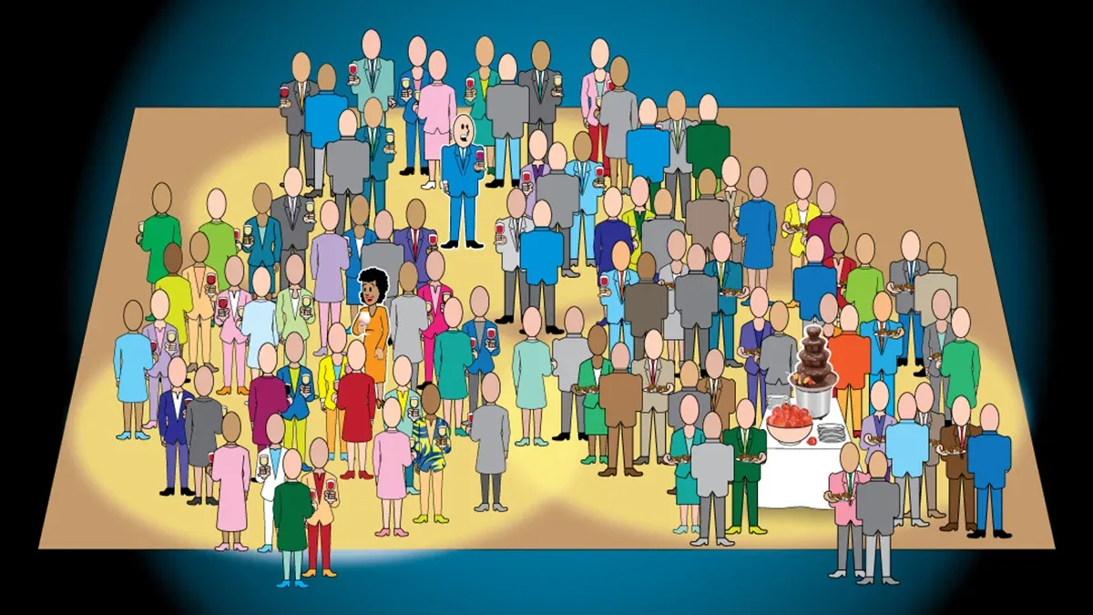
If you’re standing close to others at a party, it’s likely that you have something in common. This is the idea behind using k-means clustering to split data points into groups. Whether the groups formed via human agency or some other force, this algorithm will find them.

From detonations to dial tones: American physicist Stuart Lloyd, an alumnus of both Bell Labs’ iconic innovation factory and the Manhattan Project that invented the atomic bomb, first proposed k-means clustering in 1957 to distribute information within digital signals. He didn’t publish it until 1982. Meanwhile, American statistician Edward Forgy described a similar method in 1965, leading to its alternative name, the Lloyd-Forgy algorithm.

Finding the center: Consider breaking up the party into like-minded working groups. Given the positions of attendees in the room and the number of groups to be formed, k-means clustering can divide the attendees into groups of roughly equal size, each gathered around a central point, or centroid.

During training, the algorithm initially designates k centroids by randomly choosing k people. (K must be chosen manually, and finding an optimal value is not always trivial.) Then it grows k clusters by associating each person to the closest centroid.
For each cluster, it computes the mean position of all people assigned to the group and designates the mean position as the new centroid. Each new centroid probably isn’t occupied by a person, but so what? People tend to gather around the chocolate fondue.
Having calculated new centroids, the algorithm reassigns individuals to the centroid closest to them. Then it computes new centroids, adjusts clusters, and so on, until the centroids (and the groups around them) no longer shift. From there, assigning newcomers to the right cluster is easy. Let them take their place in the room and look for the nearest centroid.
Be forewarned: Given the initial random centroid assignments, you may not end up in the same group as that cute data-centric AI specialist you were hoping to be with. The algorithm does a good job, but it’s not guaranteed to find the best solution. Better luck at the next party!

Different distances: Of course the distance between clustered objects doesn’t need to be spatial. Any measure between two vectors will do. For instance, rather than grouping partygoers according to physical proximity, k-means clustering can divide them by their outfits, occupations, or other attributes. Online shops use it to partition customers based on their preferences or behavior, and astronomers to group stars of the same type.

Power to the data points: The idea has spawned a few notable variations:

K-medoids use actual data points as centroids rather than mean positions in a given cluster. The medoids are points that minimize the distance to all other points in their cluster. This variation is more interpretable because the centroids are always data points.
Fuzzy C-Means Clustering enables the data points to participate in multiple clusters to varying degrees. It replaces hard cluster assignments with degrees of membership depending on distance from the centroids.

Revelry in n dimensions: Nonetheless, the algorithm in its original form remains widely useful — especially because, as an unsupervised algorithm, it doesn’t require gathering potentially expensive labeled data. It’s also ever faster to use. For instance, machine learning libraries including scikit-learn benefit from the 2002 addition of kd-trees that partition high-dimensional data extremely quickly. By the way, if you throw any high-dimensional parties, we’d love to be on the guest list.